
This article is part of Quantide’s web book “Raccoon – Statistical Models with R“. Raccoon is Quantide’s third web book after “Rabbit – Introduction to R” and “Ramarro – R for Developers“. See the full project here.
The second chapter of Racooon is focused on T-test and Anova. Through example it shows theory and R code of:
- 1-sample t-test
- 2-sample t-test and Paired t
- 1-way Anova
- 2-way Anova
- Unbalanced and Nested Anova
This post is the first section of the chapter, about 1-sample t-test.
Throughout the web-book we will widely use the package qdata, containing about 80 datasets. You may find it here: https://github.com/quantide/qdata.
Ch. 2.1 – T-test, Anova: 1-sample t-test
|
1 2 3 4 5 6 7 |
require(nortest) require(car) require(ggplot2) require(dplyr) require(gridExtra) require(tidyr) require(qdata) |
Example: Reaction temperature
Data description
A chemical theory suggests that the temperature at which a certain chemical reaction occurs is 180 °C. reaction contains the results of 10 independent measurements.
Data loading
Let us load and have a look at the data
|
1 2 |
data(reaction) head(reaction) |
|
1 |
## [1] 180.6 179.4 181.3 178.5 179.8 176.9 |
|
1 |
str(reaction) |
|
1 |
## num [1:10] 181 179 181 178 180 ... |
Descriptives
First of all, let us calculate the main descriptive statistics on reaction:
|
1 2 3 4 5 6 7 8 9 10 11 12 13 |
# Add an index variable to reaction reaction <- data.frame(reaction=reaction, index=1:10) summary_stat <- reaction %>% summarise(n=n(), min=min(reaction), first_qu=quantile(reaction, 0.25), mean=mean(reaction), median=median(reaction), third_qu=quantile(reaction, 0.75), max=max(reaction), sd=sd(reaction)) print(summary_stat) |
|
1 2 |
## n min first_qu mean median third_qu max sd ## 1 10 176.9 178.725 179.49 179.6 180.55 181.3 1.427079 |
Sample mean and median are close to the hypothesized value of 180, and the data point values are close to 180 too.
Let us plot data (with collection time if meaningful) and add, with geom_hline() a reference line for temperature of 180 °C (red) and for the mean temperature (179.36 °C, green)
|
1 2 3 4 5 6 7 |
ggp <- ggplot(data = reaction, mapping=aes(x=index, y=reaction)) + geom_point() + ylim(c(177,183)) + geom_hline(yintercept = 180, color="red") + geom_hline(yintercept = mean(reaction$reaction), color="darkgreen") print(ggp) |
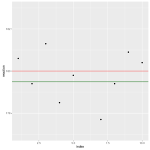
Plot of reaction values
The plot shows the temperature (y-axis) on the index of observations (x-axis). Our objective is to verify if the distance between the two lines (red and green) may be due to chance or if it is unlikely from a statistical point of view. Remember that the main objective of a statistical test is not to accept the null hypothesis, but to find if enough evidence appear to refuse it.
Now let us plot data without time (no index) by building a stripchart, which directly shows the points and is a good alternative to the boxplot:
|
1 2 3 4 5 6 7 8 9 10 11 |
reaction$index <- rep(0, times=10) ggp <- ggplot(data = reaction, mapping=aes(x=reaction, y=index)) + geom_point() + ylim(c(-2,2)) + geom_vline(xintercept = 180, color="red") + geom_vline(xintercept = mean(reaction$reaction), color="darkgreen") + ylab("") + theme(axis.text.y=element_blank(), axis.ticks=element_blank()) + annotate("text", label = "reaction mean", x = 178.8, y = 2, size = 4, colour = "darkgreen") + annotate("text", label = "target", x = 180.3, y = 2, size = 4, colour = "red") print(ggp) |
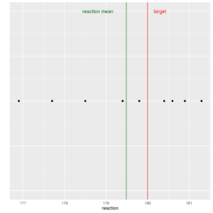
Stripchart of reaction values
Inference and models
One-sample Student’s \(t\)-test
Standard instruments, as one-sample Student’s \(t\)-test, do not use linear models at appearance. Is it true?
First let us check if the normality assumption of the \(t\)-test are plausible: let us check if data does not depart too much from normality by using the R function ad.test of the nortest require:
|
1 |
ad.test(reaction$reaction) |
|
1 2 3 4 5 |
## ## Anderson-Darling normality test ## ## data: reaction$reaction ## A = 0.25437, p-value = 0.6473 |
Anderson-Darling’s test tests the normality vs. the non-normality of data distribution. The p-value of the test is fully larger than 0.05, the usual standard for the first type
The Normal Probability Plot confirms the Anderson-Darling’s test result:
|
1 2 3 4 5 |
ggp <- ggplot(data = reaction, mapping = aes(sample = reaction)) + stat_qq(color="darkblue", size=2) + geom_abline(mapping = aes(intercept=mean(reaction),slope=sd(reaction)), color="red", linetype=2) print(ggp) |
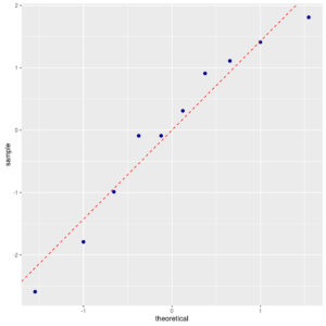
Normal probability plot of reaction
The plot compares the observed quantiles with the corresponding quantiles of a standard Normal distribution.
If data points come from a Normal distribution, then they will tendto follow a straight line.
In this case this plot is “nice”.
Now, let us test the hypothesis \(H_0\) that the “true mean is equal to 180 °C”.
|
1 |
t.test(reaction$reaction, mu = 180) |
|
1 2 3 4 5 6 7 8 9 10 11 |
## ## One Sample t-test ## ## data: reaction$reaction ## t = -1.1301, df = 9, p-value = 0.2876 ## alternative hypothesis: true mean is not equal to 180 ## 95 percent confidence interval: ## 178.4691 180.5109 ## sample estimates: ## mean of x ## 179.49 |
Linear models
How can we think to an alternative which uses a model? Since normality assumption seems satisfied, we could fit a linear model with reaction as response variable and the only intercept as parameter (the model will then report only the mean):
|
1 |
mod <- lm(formula = reaction~1, data = reaction) |
formula argument of lm function gives the “structure” of the relation between dependent and independent variables: the ~ symbol separates the dependent variable from the model formulation, and the reaction ~ 1 formula means that the dependent variable reaction is modeled by the intercept term only (the 1) , or, equivalently in this case, by the mean.The output of linear model
mod is|
1 |
mod |
|
1 2 3 4 5 6 7 |
## ## Call: ## lm(formula = reaction ~ 1, data = reaction) ## ## Coefficients: ## (Intercept) ## 179.5 |
summary() R function to lm-type objects we get more information:|
1 |
summary(mod) |
|
1 2 3 4 5 6 7 8 9 10 11 12 13 14 15 |
## ## Call: ## lm(formula = reaction ~ 1, data = reaction) ## ## Residuals: ## Min 1Q Median 3Q Max ## -2.590 -0.765 0.110 1.060 1.810 ## ## Coefficients: ## Estimate Std. Error t value Pr(>|t|) ## (Intercept) 179.4900 0.4513 397.7 <2e-16 *** ## --- ## Signif. codes: 0 '***' 0.001 '**' 0.01 '*' 0.05 '.' 0.1 ' ' 1 ## ## Residual standard error: 1.427 on 9 degrees of freedom |
|
1 2 |
reaction_z <- reaction$reaction-180 fm <- lm(reaction_z~1) |
|
1 |
fm <- lm(I(reaction-180)~1, data=reaction) |
reaction-180 has 0 mean.The output of the linear model
fm is|
1 |
summary(fm) |
|
1 2 3 4 5 6 7 8 9 10 11 12 13 |
## ## Call: ## lm(formula = I(reaction - 180) ~ 1, data = reaction) ## ## Residuals: ## Min 1Q Median 3Q Max ## -2.590 -0.765 0.110 1.060 1.810 ## ## Coefficients: ## Estimate Std. Error t value Pr(>|t|) ## (Intercept) -0.5100 0.4513 -1.13 0.288 ## ## Residual standard error: 1.427 on 9 degrees of freedom |
|
1 |
mean(reaction$reaction) - 180 |
|
1 |
## [1] -0.51 |
This particularly simple regression model is then equivalent to one-sample \(t\)-test.
Let us check for normality of residuals, even if in this particular case is redundant, since it is equivalent to check the normality of
reaction.|
1 2 |
res <- data.frame(res=fm$residuals) ad.test(res$res) |
|
1 2 3 4 5 |
## ## Anderson-Darling normality test ## ## data: res$res ## A = 0.25437, p-value = 0.6473 |
|
1 2 3 4 5 |
ggp <- ggplot(data = res, mapping = aes(sample = res)) + stat_qq(color="darkblue", size=2) + geom_abline(mapping = aes(intercept=mean(res),slope=sd(res)), color="red", linetype=2) print(ggp) |

Normal probability plot of residuals
Indeed, the p-value of Anderson-Darling’s test is the same as before. The q-q plot also confirms that the normality assumption is plausible.

[…] 1-sample t-test […]
[…] 1-sample t-test […]
[…] 1-sample t-test […]
[…] 1-sample t-test […]