
This article is part of Quantide’s web book “Raccoon – Statistical Models with R“. Raccoon is Quantide’s third web book after “Rabbit – Introduction to R” and “Ramarro – R for Developers“. See the full project here.
The second chapter of Racooon is focused on T-test and Anova. Through example it shows theory and R code of:
- 1-sample t-test
- 2-sample t-test and Paired t
- 1-way Anova
- 2-way Anova
- Unbalanced Anova with one obs dropped
- Fixed effects Nested Anova
This post is the second section of the chapter, about 2-sample t-test and paired t.
Throughout the web-book we will widely use the package qdata, containing about 80 datasets. You may find it here: https://github.com/quantide/qdata.
|
1 2 3 4 5 6 7 |
require(nortest) require(car) require(ggplot2) require(dplyr) require(gridExtra) require(tidyr) require(qdata) |
Example: Chicken hormones (2 -sample \(t\)-test)
Data description
To compare two growth hormones, 18 chicken were tested: 10 being assigned to hormone A and 8 to hormone B. The gains in weights (grams) over the period of experiment were measured.
Data loading
Let us load and have a look at the data
|
1 2 |
data(hormones) head(hormones) |
|
1 2 3 4 5 6 7 8 9 |
## # A tibble: 6 × 2 ## hormone gain ## ## 1 A 615 ## 2 A 645 ## 3 A 840 ## 4 A 645 ## 5 A 365 ## 6 A 450 |
|
1 |
str(hormones) |
|
1 2 3 |
## Classes 'tbl_df', 'tbl' and 'data.frame': 18 obs. of 2 variables: ## $ hormone: Factor w/ 2 levels "A","B": 1 1 1 1 1 1 1 1 1 1 ... ## $ gain : int 615 645 840 645 365 450 530 756 785 560 ... |
Descriptives
We begin by calculating some descriptive statistics:
|
1 2 3 4 5 6 7 8 |
hormones %>% group_by(hormone) %>% summarise(min = min(gain), first_qu = quantile(gain, 0.25), median = median(gain), mean = mean(gain), third_qu = quantile(gain, 0.75), max = max(gain), sd = sd(gain)) |
|
1 2 3 4 5 |
## # A tibble: 2 × 8 ## hormone min first_qu median mean third_qu max sd ## ## 1 A 365 537.5 630.0 619.100 728.25 840 149.4482 ## 2 B 560 742.0 827.5 822.625 916.25 1035 154.5574 |
And now we draw a boxplot and a stripchart (in this case in vertical) of the data:
|
1 2 3 4 |
ggp <- ggplot(data = hormones, mapping = aes(x=hormone, y=gain, fill=hormone)) + geom_boxplot() print(ggp) |
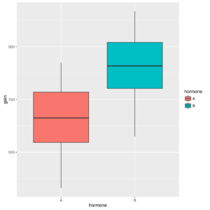
Box-and-whiskers plot of gain by hormone
|
1 2 3 4 5 6 7 8 |
hormones_mean <- hormones %>% group_by(hormone) %>% summarise(gain=mean(gain)) ggp <- ggplot(data = hormones, mapping = aes(x=hormone, y=gain)) + geom_jitter(position = "dodge", color="darkblue") + geom_point(data=hormones_mean, mapping = aes(x=hormone,y=gain), colour="red", group=1) + geom_line(data=hormones_mean, mapping = aes(x=hormone,y=gain), colour="red", group=1) print(ggp) |
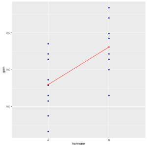
Stripchart with connect line of gain by hormone
The geom_point() function and geom_line() functions add the red points of two group averages to second graph and then link them with a segment.
group_by() and summarise() functions applies separately the mean() function to values of gain corresponding to hormone variable levels. In this case, if the segment is near to parallel to the x-axis, then the two means are probably equal. Anyway, both graphs and statistics show that hormone B tends to generate heavier chickens.
Inference and models
Let us check the normality of gain in the two groups through q-q plots
|
1 2 3 4 5 6 7 8 9 10 11 12 13 14 |
hormones_a <- hormones %>% filter(hormone =="A") hormones_b <- hormones %>% filter(hormone =="B") ggp1 <- ggplot(data = hormones_a, mapping = aes(sample = gain)) + stat_qq(color="#F8766D", size=2) + geom_abline(intercept=mean(hormones_a$gain),slope=sd(hormones_a$gain), color="red", linetype=2) + ylab("hormone A") + ggtitle("q-q plot of hormone A") ggp2 <- ggplot(data = hormones_b, mapping = aes(sample = gain)) + stat_qq(color="#00C094", size=2) + geom_abline(mapping = aes(intercept=mean(hormones_b$gain),slope=sd(hormones_b$gain)), color="red", linetype=2) + ylab("hormone B") + ggtitle("q-q plot of hormone B") grid.arrange(ggp1, ggp2, nrow = 2) |
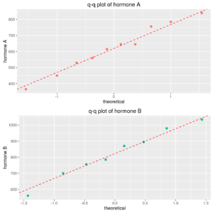
Normal probability plot of gain by hormone
From graph, no evidence of non-normality is evident. Now let us perform Anderson-Darling’s test for gain in the two groups, exploiting the function tapply:
|
1 |
tapply(hormones$gain, hormones$hormone, ad.test) |
|
1 2 3 4 5 6 7 8 9 10 11 12 13 14 |
## $A ## ## Anderson-Darling normality test ## ## data: X[[i]] ## A = 0.15886, p-value = 0.926 ## ## ## $B ## ## Anderson-Darling normality test ## ## data: X[[i]] ## A = 0.13781, p-value = 0.9557 |
The last line of above code, returns a 2-element list, with AD test for each sub-group. There is no evidence to reject the normality hypothesis within the two groups.
The next line of code tests the homoscedasticity assumption, that is if the variances within the two groups are equal:
|
1 |
var.test(gain ~ hormone, data = hormones) |
|
1 2 3 4 5 6 7 8 9 10 11 |
## ## F test to compare two variances ## ## data: gain by hormone ## F = 0.93498, num df = 9, denom df = 7, p-value = 0.9031 ## alternative hypothesis: true ratio of variances is not equal to 1 ## 95 percent confidence interval: ## 0.1938497 3.9241513 ## sample estimates: ## ratio of variances ## 0.9349792 |
|
1 |
bartlett.test(gain ~ hormone,data=hormones) |
|
1 2 3 4 5 |
## ## Bartlett test of homogeneity of variances ## ## data: gain by hormone ## Bartlett's K-squared = 0.0083868, df = 1, p-value = 0.927 |
|
1 |
leveneTest(gain ~ hormone,data=hormones) |
|
1 2 3 4 |
## Levene's Test for Homogeneity of Variance (center = median) ## Df F value Pr(>F) ## group 1 0.0321 0.8601 ## 16 |
All three previous tests accept \(H_0\), i.e., there is no evidence to say that the variability changes across levels.
Now the \(t\)-test compares the two group means.
The null hypothesis is \(H_0: beta_1 = beta_2\), where \(beta_1\) and \(beta_2\) are the expectations of dependent variable for hormones A and B, respectively.
|
1 |
t.test(gain ~ hormone, data = hormones, var.equal = TRUE) |
|
1 2 3 4 5 6 7 8 9 10 11 |
## ## Two Sample t-test ## ## data: gain by hormone ## t = -2.8283, df = 16, p-value = 0.01211 ## alternative hypothesis: true difference in means is not equal to 0 ## 95 percent confidence interval: ## -356.07303 -50.97697 ## sample estimates: ## mean in group A mean in group B ## 619.100 822.625 |
The \(t\)-test rejects the null hypothesis.
Now the same test may be conducted using a model approach.
The following lines of code perform the model fitting and print the main results.
|
1 2 |
mod <- lm(gain ~ hormone, data = hormones) mod |
|
1 |
## |
|
1 2 3 4 5 6 |
## Call: ## lm(formula = gain ~ hormone, data = hormones) ## ## Coefficients: ## (Intercept) hormoneB ## 619.1 203.5 |
The parameters shown are the model intercept and the “slope” coefficient for hormone B. The intercept in this case is the estimate of mean growth for A hormone, whereas the slope in this case is the estimate of difference between the mean growth obtained with hormon B and the mean growth obtained with hormone A.
In other words, the mean growth estimate for hormoneA is 619.1, while the mean growth estimate for hormoneB is 619.1 + 203.5 = 822.6. We will return to parameterization issue later.
Using summary the significancy of parameters is also shown:
|
1 |
summary(mod) |
|
1 2 3 4 5 6 7 8 9 10 11 12 13 14 15 16 17 18 |
## ## Call: ## lm(formula = gain ~ hormone, data = hormones) ## ## Residuals: ## Min 1Q Median 3Q Max ## -262.62 -83.48 10.90 120.77 220.90 ## ## Coefficients: ## Estimate Std. Error t value Pr(>|t|) ## (Intercept) 619.10 47.97 12.905 7.12e-10 *** ## hormoneB 203.53 71.96 2.828 0.0121 * ## --- ## Signif. codes: 0 '***' 0.001 '**' 0.01 '*' 0.05 '.' 0.1 ' ' 1 ## ## Residual standard error: 151.7 on 16 degrees of freedom ## Multiple R-squared: 0.3333, Adjusted R-squared: 0.2916 ## F-statistic: 7.999 on 1 and 16 DF, p-value: 0.01211 |
The test results are equal to the ones of \(t\)-test, and the \(t\)-test value is equal to minus \(t\)-test value of hormoneB coefficient.
Why these results? “Behind the scene”, the model has been built using the following **model matrix** (\(underline{X}\))
|
1 |
model.matrix(mod) |
|
1 2 3 4 5 6 7 8 9 10 11 12 13 14 15 16 17 18 19 20 21 22 23 24 |
## (Intercept) hormoneB ## 1 1 0 ## 2 1 0 ## 3 1 0 ## 4 1 0 ## 5 1 0 ## 6 1 0 ## 7 1 0 ## 8 1 0 ## 9 1 0 ## 10 1 0 ## 11 1 1 ## 12 1 1 ## 13 1 1 ## 14 1 1 ## 15 1 1 ## 16 1 1 ## 17 1 1 ## 18 1 1 ## attr(,"assign") ## [1] 0 1 ## attr(,"contrasts") ## attr(,"contrasts")$hormone ## [1] "contr.treatment" |
What this matrix means?
For modeling purposes, the independent variable hormone has been “split” in two dummy variables: hormoneA and hormoneB:
hormoneAis1when data contain measures relative to hormoneA, and is0when data contain measures relative to hormoneBhormoneBis1when data contain measures relative to hormoneB, and is0when data contain measures relative to hormoneA
Obviously, when hormoneA is 0, hormoneB is 1 and vice versa. Then, one dummy variable (in this case, hormoneA), can be removed from the model, because it does not add any useful information, and makes the model mathematically non-manageable. Consequently, the model matrix will contains only the “all 1s” intercept column (that refers to the case when hormone A is used) and the “displacement” hormoneBcolumn which represents the constant added to mean growth when using hormone B instead of hormone A.
In other words, the model actually estimated is the following:
\( growth_i = beta_0 + beta_1 cdot delta_B(hormone_i) + varepsilon_i \)
Where \(delta_B(hormone_i)\) represents the function that returns 1 only when the hormone of \(i\)-th unit is B, otherwise, returns 0.
\(beta_0\) in this manner is the value of mean growth when using hormone A (i.e., when \(delta_B(hormone_i)==0\)), while \(beta_1\) is the “jump” in mean of growth when using hormone B instead of hormone A.
Another approach available to manage such type of test is through the analysis of variance model, i.e. by using the aov() function, that directly performs one analysis of variance:
|
1 |
fm <- aov(mod) |
Printing a summary method for analysis of variance objects reflects the different approach to what is essentially the same information as returned by lm(). While a printed linear-model object shows individual coefficients, printed aov objects show terms, which may correspond to several coefficients. However, methods for linear models can always be applied explicitly on aov objects, such as those for the coefficients or residuals.
|
1 |
summary(fm) |
|
1 2 3 4 5 |
## Df Sum Sq Mean Sq F value Pr(>F) ## hormone 1 184100 184100 7.999 0.0121 * ## Residuals 16 368229 23014 ## --- ## Signif. codes: 0 '***' 0.001 '**' 0.01 '*' 0.05 '.' 0.1 ' ' 1 |
Above output shows that hormone, with all its levels, is globally significant (p=0.012) in explaining the dependent variable variability.
In this case, since the independent variable (factor) contains two levels only, the resulting p-value for hormone obtained from aov is identical to the p-value of hormone B obtained using lm() (actually, in this example they are the same test).
If the independent variable (factor) contains more than two levels, then aov() returns the global significancy (not the “by level significancy”) of independent variable effect on dependent variable.
A few more concise code to obtain the same results as above is
|
1 2 |
fm <- aov(gain ~ hormone, data = hormones) summary(fm) |
|
1 2 3 4 5 |
## Df Sum Sq Mean Sq F value Pr(>F) ## hormone 1 184100 184100 7.999 0.0121 * ## Residuals 16 368229 23014 ## --- ## Signif. codes: 0 '***' 0.001 '**' 0.01 '*' 0.05 '.' 0.1 ' ' 1 |
Next lines of code show that actually aov objects are lm objects with also analysis of variance results added.
|
1 |
class(mod) |
|
1 |
## [1] "lm" |
|
1 |
class(fm) |
|
1 |
## [1] "aov" "lm" |
The following commands are useful to read/define the type of contrasts (i.e., the type of coding of regressors matrix \(underline{X}\)) used when unordered or ordered factors are used.
|
1 |
options("contrasts") |
|
1 2 3 |
## $contrasts ## unordered ordered ## "contr.treatment" "contr.poly" |
|
1 |
options(contrasts = c("contr.treatment", "contr.poly")) |
The first line of code simply shows the current predefined type of contrasts for unordered and ordered factors, while the second line of code sets the predefined contrasts.
To extract coefficients from an already calculated (lm or aov) model, one must use the coefficients method:
|
1 |
coefficients(fm) |
|
1 2 |
## (Intercept) hormoneB ## 619.100 203.525 |
Next line of code shows that the hormoneB coefficient is simply the difference between average growths for hormoneA and hormoneB chickens.
|
1 |
diff(tapply(hormones$gain, hormones$hormone, mean)) |
|
1 2 |
## B ## 203.525 |
R can use several types of contrasts: contr.treatment sets to zero the coefficient of first factor level, that becomes the intercept, and consequently all the means of other levels are relative to the first level. Another option is contr.sum, that sets to zero the sum of coefficients, and then the reference value of coefficients becomes the gran mean, calculated on all factor levels. R uses contr.treatment as default.
Let’s try to change type of contrasts:
|
1 |
options(contrasts = c("contr.sum", "contr.poly")) |
|
1 |
fm <- aov(gain~hormone, data = hormones) |
The aov() results are the same:
|
1 |
summary(fm) |
|
1 2 3 4 5 |
## Df Sum Sq Mean Sq F value Pr(>F) ## hormone 1 184100 184100 7.999 0.0121 * ## Residuals 16 368229 23014 ## --- ## Signif. codes: 0 '***' 0.001 '**' 0.01 '*' 0.05 '.' 0.1 ' ' 1 |
but, on the whole, the results are changed:
|
1 |
coefficients(fm) |
|
1 2 |
## (Intercept) hormone1 ## 720.8625 -101.7625 |
The values of the coefficients are not the same because with contr.treatment the intercept represents the mean in the first group (hormone A) and the “slope” represents the difference between the mean in the second group (hormone B) and the mean in the first group; conversely, with contr.sum the intercept represents the grand mean, and the slope represents the difference between the mean in the first group and the grand mean.
The differences in coefficients are perhaps more perceptible looking at the model matrix:
|
1 |
model.matrix(fm) |
|
1 2 3 4 5 6 7 8 9 10 11 12 13 14 15 16 17 18 19 20 21 22 23 24 |
## (Intercept) hormone1 ## 1 1 1 ## 2 1 1 ## 3 1 1 ## 4 1 1 ## 5 1 1 ## 6 1 1 ## 7 1 1 ## 8 1 1 ## 9 1 1 ## 10 1 1 ## 11 1 -1 ## 12 1 -1 ## 13 1 -1 ## 14 1 -1 ## 15 1 -1 ## 16 1 -1 ## 17 1 -1 ## 18 1 -1 ## attr(,"assign") ## [1] 0 1 ## attr(,"contrasts") ## attr(,"contrasts")$hormone ## [1] "contr.sum" |
Now, firstly we will restore predefined contrasts
|
1 |
options(contrasts = c("contr.treatment", "contr.poly")) |
and then we will fit a model without intercept to data. In general, removing the intercept is a discouraged practice, but sometimes no intercept models can help to enhance coefficients meaning:
|
1 2 |
mod <- lm(gain ~ hormone-1, data = hormones) coefficients(mod) |
|
1 2 |
## hormoneA hormoneB ## 619.100 822.625 |
The above coefficients represent, respectively, the mean in the group hormoneA and in the group hormoneB.
The model matrix can be useful to understand the meaning of the coefficients:
|
1 |
model.matrix(mod) |
|
1 2 3 4 5 6 7 8 9 10 11 12 13 14 15 16 17 18 19 20 21 22 23 24 |
## hormoneA hormoneB ## 1 1 0 ## 2 1 0 ## 3 1 0 ## 4 1 0 ## 5 1 0 ## 6 1 0 ## 7 1 0 ## 8 1 0 ## 9 1 0 ## 10 1 0 ## 11 0 1 ## 12 0 1 ## 13 0 1 ## 14 0 1 ## 15 0 1 ## 16 0 1 ## 17 0 1 ## 18 0 1 ## attr(,"assign") ## [1] 1 1 ## attr(,"contrasts") ## attr(,"contrasts")$hormone ## [1] "contr.treatment" |
Next code shows what can happen when one uses a no-intercept model and does not address for that in analysis of variance:
|
1 2 |
fm <- aov(mod) summary(fm) |
|
1 2 3 4 5 |
## Df Sum Sq Mean Sq F value Pr(>F) ## hormone 2 9246543 4623272 200.9 4.63e-12 *** ## Residuals 16 368229 23014 ## --- ## Signif. codes: 0 '***' 0.001 '**' 0.01 '*' 0.05 '.' 0.1 ' ' 1 |
|
1 |
coefficients(fm) |
|
1 2 |
## hormoneA hormoneB ## 619.100 822.625 |
The significancy of factor is much more strong than in previous calculations, but this is wrong, because this result actually compares the model with 0 intercept with the model that uses one mean for hormoneAand one mean for hormoneB.
Using the following code gives results equivalent to t-test:
|
1 |
anova(mod,lm(gain ~ 1, data = hormones)) |
|
1 2 3 4 5 6 7 8 9 |
## Analysis of Variance Table ## ## Model 1: gain ~ hormone - 1 ## Model 2: gain ~ 1 ## Res.Df RSS Df Sum of Sq F Pr(>F) ## 1 16 368229 ## 2 17 552328 -1 -184100 7.9994 0.01211 * ## --- ## Signif. codes: 0 '***' 0.001 '**' 0.01 '*' 0.05 '.' 0.1 ' ' 1 |
anova() performs an analysis of variance to compare two nested models (see the paragraph on Comparing two nested models in Some Theory on Linear Models chapter).
In this case we are comparing a model with the group variable hormone against the model with grand mean only.
The result is the same as seen individually in lm() and aov() outputs.
Model diagnostics
Since the assumpions on linear models, the residuals should arise from a gaussian distribution; then, a Normal Probability Plot of residuals will be plotted to check this assumption.
|
1 2 3 |
res <- cbind(hormones,res=fm$residuals) ad.test(res$res) |
|
1 2 3 4 5 |
## ## Anderson-Darling normality test ## ## data: res$res ## A = 0.18963, p-value = 0.8859 |
|
1 2 3 4 5 |
ggp <- ggplot(data = res, mapping = aes(sample = res, color=hormone)) + stat_qq(size=2) + geom_abline(mapping = aes(intercept=mean(res), slope=sd(res)), colour="red", linetype=2) print(ggp) |
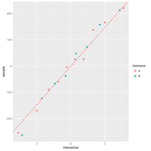
Overlaid Normal probability plots of residuals
The two colors correspond to two groups.
Residuals seem gaussian, irrespective of group.
The Anderson-Darling (AD) test confirms that:
|
1 |
ad.test(fm$residuals) |
|
1 2 3 4 5 |
## ## Anderson-Darling normality test ## ## data: fm$residuals ## A = 0.18963, p-value = 0.8859 |
This confirms that the analysis and its results may be considered correct.
Example: Park assistant (paired \(t\))
Data description
In an experiment to investigate if an optional equipment of cars may help to park the cars themselves, 20 drivers were asked to park the car with and without the equipment. The parking time (secs) for each driver and equipment is recorded.
Data loading
|
1 2 |
data(carctl) str(carctl) |
|
1 2 3 |
## Classes 'tbl_df', 'tbl' and 'data.frame': 20 obs. of 2 variables: ## $ Car_A: num 35.4 28.9 32.1 40.6 18.3 ... ## $ Car_B: num 28.6 24.4 37.3 39.9 21.7 ... |
Descriptives
A simple boxplot:
|
1 |
carctl2 % gather(car, value, Car_A, Car_B) |
|
1 2 3 4 |
ggp <- ggplot(data = carctl2, mapping = aes(x=car, y=value, fill=car)) + geom_boxplot() print(ggp) |
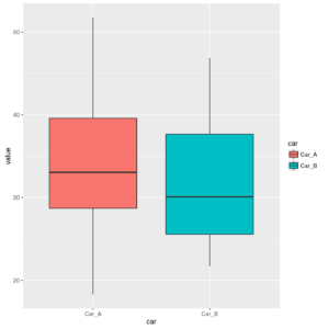
Box-and-whiskers plot of parking times for the two cars
A stripchart with mean points and mean line:
|
1 |
carctl_mean % group_by(car) %>% summarise(value=mean(value)) |
|
1 2 3 4 5 6 |
ggp <- ggplot(data = carctl2, mapping = aes(x=car, y=value)) + geom_jitter(position = "dodge", color="darkblue") + geom_point(data=carctl_mean, mapping = aes(x=car,y=value), colour="red", group=1) + geom_line(data=carctl_mean, mapping = aes(x=car,y=value), colour="red", group=1) print(ggp) |
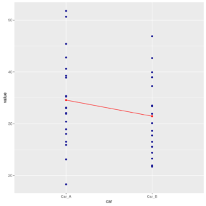
Stripchart with connect line of parking times for the two cars
And now the \(t\)-test.
Before testing the means, a check for normality is made by using qq-plot and Anderson-Darling test
|
1 2 3 4 5 6 |
ggp <- ggplot(data = carctl2, mapping = aes(sample = value, color=car)) + stat_qq() + geom_abline(data= carctl2 %>% filter(car=="Car_A"), mapping=aes(intercept=mean(value), slope=sd(value), color=car), size=1) + geom_abline(data= carctl2 %>% filter(car=="Car_B"), mapping=aes(intercept=mean(value), slope=sd(value), color=car), size=1) |
|
1 |
print(ggp) |
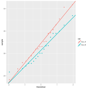
Normal probability plot of parking times of two cars
There is not evidence of non-normality within groups, and the AD tests confirm above results:
|
1 |
lapply(X=carctl, FUN=ad.test) |
|
1 2 3 4 5 6 7 8 9 10 11 12 13 14 |
## $Car_A ## ## Anderson-Darling normality test ## ## data: X[[i]] ## A = 0.19988, p-value = 0.8647 ## ## ## $Car_B ## ## Anderson-Darling normality test ## ## data: X[[i]] ## A = 0.36913, p-value = 0.3928 |
and finally the two independent samples \(t\)-test:
|
1 |
t.test(x=carctl$Car_A, y=carctl$Car_B) |
|
1 2 3 4 5 6 7 8 9 10 11 |
## ## Welch Two Sample t-test ## ## data: carctl$Car_A and carctl$Car_B ## t = 1.2205, df = 36.778, p-value = 0.2301 ## alternative hypothesis: true difference in means is not equal to 0 ## 95 percent confidence interval: ## -2.056978 8.285186 ## sample estimates: ## mean of x mean of y ## 34.56418 31.45008 |
Following this result, the null hypothesis is not rejected (at a 5% level).
But if we produce a scatterplot of Car_A Vs Car_B,
|
1 2 3 4 |
ggp <- ggplot(data = carctl, mapping = aes(x=Car_A, y=Car_B)) + geom_point(col="darkblue") print(ggp) |
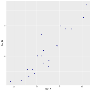
Scattrplot of parking times of Car_A Vs. Car_B
we can see that data of two cars are clearly NOT independent!!
Measures on Car_A are strongly related to measures on Car_B, because each driver drove either cars.
Then the correct test for such as data is:
|
1 2 |
carctl % mutate(car_diff = Car_A - Car_B) t.test(x=carctl$car_diff, mu=0) |
|
1 2 3 4 5 6 7 8 9 10 11 |
## ## One Sample t-test ## ## data: carctl$car_diff ## t = 3.8735, df = 19, p-value = 0.001023 ## alternative hypothesis: true mean is not equal to 0 ## 95 percent confidence interval: ## 1.431407 4.796801 ## sample estimates: ## mean of x ## 3.114104 |
or, equivalently, a paired \(t\)-test(x=carctl\(Car_A, y=carctl\)Car_B, paired=TRUE)
|
1 |
t.test(x=carctl$Car_A, y=carctl$Car_B, paired=TRUE) |
|
1 2 3 4 5 6 7 8 9 10 11 |
## ## Paired t-test ## ## data: carctl$Car_A and carctl$Car_B ## t = 3.8735, df = 19, p-value = 0.001023 ## alternative hypothesis: true difference in means is not equal to 0 ## 95 percent confidence interval: ## 1.431407 4.796801 ## sample estimates: ## mean of the differences ## 3.114104 |
In either cases the results are the same: a difference statistically significant exists between mean parking times of two cars.
In this case the Normality test must be performed on differences between measures within same driver.
Check of normality by Normal probability plot:
|
1 2 3 4 5 |
ggp <- ggplot(data = carctl, mapping = aes(sample = car_diff)) + stat_qq(color="darkblue", size=2) + geom_abline(mapping = aes(intercept=mean(car_diff), slope=sd(car_diff)), colour="red", linetype=2) print(ggp) |
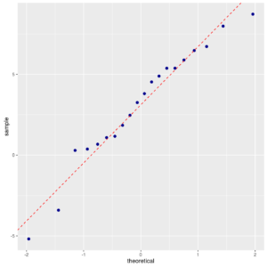
Normal probability plot of difference of parking times of two cars
And the Anderson-Darling test:
|
1 |
ad.test(x=carctl$car_diff) |
|
1 2 3 4 5 |
## ## Anderson-Darling normality test ## ## data: carctl$car_diff ## A = 0.29177, p-value = 0.5704 |
For either tests, the Normality assumption is not rejected.
Now we try the model approach to the same test. The model approach in this case follows the same procedure seen for the one-sample t-test, but using the differences between times as dependent variable.
Fitting of model:
|
1 2 |
mod <- lm(car_diff ~ 1, data = carctl) mod |
|
1 2 3 4 5 6 7 |
## ## Call: ## lm(formula = car_diff ~ 1, data = carctl) ## ## Coefficients: ## (Intercept) ## 3.114 |
|
1 |
summary(mod) |
|
1 2 3 4 5 6 7 8 9 10 11 12 13 14 15 |
## ## Call: ## lm(formula = car_diff ~ 1, data = carctl) ## ## Residuals: ## Min 1Q Median 3Q Max ## -8.2986 -2.1332 0.4141 2.3877 5.6064 ## ## Coefficients: ## Estimate Std. Error t value Pr(>|t|) ## (Intercept) 3.114 0.804 3.873 0.00102 ** ## --- ## Signif. codes: 0 '***' 0.001 '**' 0.01 '*' 0.05 '.' 0.1 ' ' 1 ## ## Residual standard error: 3.595 on 19 degrees of freedom |
or, equivalently one may use also:
|
1 2 |
mod <- lm(I(Car_A-Car_B)~1, data=carctl) summary(mod) |
|
1 2 3 4 5 6 7 8 9 10 11 12 13 14 15 |
## ## Call: ## lm(formula = I(Car_A - Car_B) ~ 1, data = carctl) ## ## Residuals: ## Min 1Q Median 3Q Max ## -8.2986 -2.1332 0.4141 2.3877 5.6064 ## ## Coefficients: ## Estimate Std. Error t value Pr(>|t|) ## (Intercept) 3.114 0.804 3.873 0.00102 ** ## --- ## Signif. codes: 0 '***' 0.001 '**' 0.01 '*' 0.05 '.' 0.1 ' ' 1 ## ## Residual standard error: 3.595 on 19 degrees of freedom |
q-q plot (or Normal probability plot) of residuals shall be identical to previous one.
The Anderson-Darling test too is identical to previuosly made test:
|
1 |
ad.test(mod$residuals) |
|
1 2 3 4 5 |
## ## Anderson-Darling normality test ## ## data: mod$residuals ## A = 0.29177, p-value = 0.5704 |
equivalently:
|
1 |
ad.test(residuals(mod)) |
|
1 2 3 4 5 |
## ## Anderson-Darling normality test ## ## data: residuals(mod) ## A = 0.29177, p-value = 0.5704 |
Note that for repeated measures experiments, several analytical options are also available: for example through the Error() function in formula specification, or using mixed-model methods (lme4 or nlmepackages are the most used and known).
In this manual we won’t deep these arguments, because they would require a distinct section for each of them.

[…] 2-sample t-test and Paired t […]
[…] 2-sample t-test and Paired t […]