Raccoon | Ch 2.3 – 1-way Anova

This article is part of Quantide’s web book “Raccoon – Statistical Models with R“. Raccoon is Quantide’s third web book after “Rabbit – Introduction to R” and “Ramarro – R for Developers“. See the full project here.

The second chapter of Raccoon is focused on T-test and Anova. Through example it shows theory and R code of:

• 1-sample t-test
• 2-sample t-test and Paired t
• 1-way Anova
• 3-way Anova
• Unbalanced and Nested

This post is the third section of the chapter, about 1-way Anova.

Throughout the web-book we will widely use the package qdata, containing about 80 datasets. You may find it here: https://github.com/quantide/qdata.

Example: Tissues (1-way ANOVA)

Data description

Three quality inspectors of a plant, Henry, Anne, and Andrew (operators) measure the strenght of car seat tissues. The company managers want to test the reproducibility, between operators, of company’s measurement system.
The main goal of study is then to verify if operators’ measures are confrontable.
Each operator measured 25 pieces of car seat tissues.
Globally, 75 samples of tissue randomly chosen from the same production batch were measured.

Data loading

Data is already ordered by operator (Anne, Henry, and Andrew)

Descriptives

Plot of Strengt with Operator factor variable in abscissa:

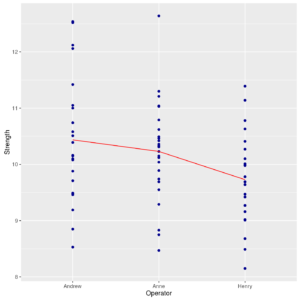
Stripchart of Strenght by Operator with connect line

A different way to show similar information is through a plot of univariate effects:

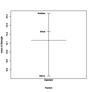Plot of univariate effects of Operator on Strenght

This plot shows the mean for each level of grouping factor compared to the grand mean (the center wider line).

Inference and models

Now we will try models with different contrast types.
Initially the model with default contrasts will be fitted to data, then the contr.sum and the contr.helmert contrast models will be shown.

Default contrasts:

aov()’s predefined output gives a global p-value of 0.0258 on Operator effect.

Note that summary.lm() shows the aov resulting object fm_treatment as if it simply were an lm-type object.

From its output, Andrew’s mean appears significantly different from 0 (\(beta_0\) = 10.4364, p = 2e-16),

Henry seems significantly different from Andrew (0.7076 lesser, p-value=0.00868), whereas Anne’s seem not significantly different from Andrew (0.2064 lesser, p-value=0.43384).  

Instead of summary() and summary.lm(), summary.aov() and summary() may be used, obtaining the same outputs:

In this sense, aov(),lm() and their resulting objects are substantially interchangeable.

Now let’s see what changes if constrasts settings are modified. The first contrast setting is contr.sum:

The interpretation of the contr.sum coefficients is not very simple: contrasts are the \(k-1\) differences (where \(k\) is the number of factor levels) between each level and a reference level; the resulting estimated coefficients contain the differences of each level mean (excluded the reference level) with respect to the grand mean; in fact, the model intercept is equal to grand mean.  

aov(), however, gives the same results obtained with default contrasts.

Now let’s change contrast settings by selecting Helmert contrasts

Helmert’s contrasts are even more complex than the others; they analyze:  

1. Initially, the difference between first level mean and the second level mean
2. Then, the difference between the mean of first two (pooled) levels and the third level mean
3. Then, the difference between the mean of first three (pooled) levels and the fourth level mean
4. And so on for \(k-1\) contrasts

The main advantage of using Helmert contrasts is that they are orthogonal; the tests on linear model coefficients are then stocastically independent: the Type I and Type II error rate for the tests on Helmert coefficients are unrelated. The main disavantage, of course, is their complexity in coefficients explanations.

Now, let’s restore predefined contrasts:

Summarizing the results just seen about contrasts:

• contr.treatment makes easier to read results, but the tests on coefficients are NOT independent
• contr.sum makes NO independent tests on coefficients, but compares pairs of means; also, the coefficients represent the distance of level’s mean with respect to grand mean, however they are not always easily interpretable
• contr.helmert makes independent tests on coefficients, but the coefficients are more difficult to interpret
• anyway, until now, the global ANOVA (aov())results are always the same: aov() analyzes effects globally, not single means

Residuals analysis

By plotting a model object (lm or aov) up to six residuals diagnostic plots may be shown.

By default, the plot() method applied on a model object shows four graphs:

1. A plot of raw residuals against fitted values
2. A Normal Q-Q plot on standardized residuals
3. A scale-Location plot of \(sqrt{vert std. residuals vert}\) against fitted values. Here, \(std. residuals\) means raw residuals divided by \(hatsigma cdot sqrt{1-h_{ii}}\), where \(h_{ii}\) are the diagonal entries of the “hat” matrix (see Appendices chapter).
4. A plot of standardized Pearson residuals against leverages. If the leverages are constant (as is the case in the balanced design of this example) the plot uses factor level combinations instead of the leverages for the x-axis.

The next lines of code split the graphical device in 4 areas (2 x 2) and plot diagnostic graphs in only one display

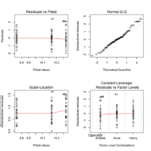
Compound diagnostic residual plot of Strenght Vs. Operator ANOVA model

The last line of above code restores the graphical device.

The residual plots confirm that normality and homoscedasticity assumptions are met, and no outliers appear. This confirms the model results.