Principal components regression (PCR) is a regression technique based on principal component analysis (PCA).
The basic idea behind PCR is to calculate the principal components and then use some of these components as predictors in a linear regression model fitted using the typical least squares procedure.
As you can easily notice, the core idea of PCR is very closely related to the one underlying PCA and the “trick” is very similar. In some cases a small number of principal components are enough to explain the vast majority of the variability in the data. For instance, say you have a dataset of 50 variables that you would like to use to predict a single variable. By using PCR you might found out that 4 or 5 principal components are enough to explain 90% of the variance of your data. In this case, you might be better off running PCR on with these 5 components instead of running a linear model on all the 50 variables. This is a rough example but I hope it helped to get the point through.
A core assumption of PCR is that the directions in which the predictors show the most variation are the exact directions associated with the response variable. On one hand, this assumption is not guaranteed to hold 100% of the times, however, even though the assumption is not completely true it can be a good approximation and yield interesting results.
Some of the most notable advantages of performing PCR are the following:
- Dimensionality reduction
- Avoidance of multicollinearity between predictors
- Overfitting mitigation
Let’s briefly walk through each one of them:
Dimensionality reduction
By using PCR you can easily perform dimensionality reduction on a high dimensional dataset and then fit a linear regression model to a smaller set of variables, while at the same time keep most of the variability of the original predictors. Since the use of only some of the principal components reduces the number of variables in the model, this can help in reducing the model complexity, which is always a plus. In case you need a lot of principal components to explain most of the variability in your data, say roughly as many principal components as the number of variables in your dataset, then PCR might not perform that well in that scenario, it might even be worse than plain vanilla linear regression.
PCR tends to perform well when the first principal components are enough to explain most of the variation in the predictors.
Avoiding multicollinearity
A significant benefit of PCR is that by using the principal components, if there is some degree of multicollinearity between the variables in your dataset, this procedure should be able to avoid this problem since performing PCA on the raw data produces linear combinations of the predictors that are uncorrelated.
Overfitting mitigation
If all the assumptions underlying PCR hold, then fitting a least squares model to the principal components will lead to better results than fitting a least squares model to the original data since most of the variation and information related to the dependent variable is condensend in the principal components and by estimating less coefficients you can reduce the risk of overfitting.
Potential drawbacks and warnings
As always with potential benefits come potential risks and drawbacks.
For instance, a typical mistake is to consider PCR a feature selection method. PCR is not a feature selection method because each of the calculated principal components is a linear combination of the original variables. Using principal components instead of the actual features can make it harder to explain what is affecting what.
Another major drawback of PCR is that the directions that best represent each predictor are obtained in an unsupervised way. The dependent variable is not used to identify each principal component direction. This essentially means that it is not certain that the directions found will be the optimal directions to use when making predictions on the dependent variable.
Performing PCR on a test dataset
There are a bunch of packages that perform PCR however, in my opinion, the pls package offers the easiest option. It is very user friendly and furthermore it can perform data standardization too. Let’s make a test.
Before performing PCR, it is preferable to standardize your data. This step is not necessary but strongly suggested since PCA is not scale invariant. You might ask why is it important that each predictor is on the same scale as the others. The scaling will prevent the algorithm to be skewed towards predictors that are dominant in absolute scale but perhaps not so relevant as others. In other words, variables with higher variance will influence more the calculation of the principal components and overall have a larger effect on the final results of the algorithm. Personally I would prefer to standardize the data most of the times.
Another thing to assess before running PCR is missing data: you should remove all the observations containing missing data, or approximate the missing observations with some technique before running the PCR function.
For this toy example, I am using the evergreen iris dataset.
|
1 2 3 4 |
require(pls) set.seed (1000) pcr_model <- pcr(Sepal.Length~., data = iris, scale = TRUE, validation = "CV") |
By setting the parameter scale equal to TRUE the data is standardized before running the pcr algorithm on it. You can also perform validation by setting the argument validation. In this case I chose to perform 10 fold cross-validation and therefore set the validation argument to “CV”, however there other validation methods available just type ?pcr in the R command window to gather some more information on the parameters of the pcr function.
In oder to print out the results, simply use the summary function as below
|
1 |
summary(pcr_model) |
|
1 2 3 4 5 6 7 8 9 10 11 12 13 14 15 |
## Data: X dimension: 150 5 ## Y dimension: 150 1 ## Fit method: svdpc ## Number of components considered: 5 ## ## VALIDATION: RMSEP ## Cross-validated using 10 random segments. ## (Intercept) 1 comps 2 comps 3 comps 4 comps 5 comps ## CV 0.8308 0.5141 0.5098 0.3947 0.3309 0.3164 ## adjCV 0.8308 0.5136 0.5092 0.3941 0.3303 0.3156 ## ## TRAINING: % variance explained ## 1 comps 2 comps 3 comps 4 comps 5 comps ## X 56.20 88.62 99.07 99.73 100.00 ## Sepal.Length 62.71 63.58 78.44 84.95 86.73 |
As you can see, two main results are printed, namely the validation error and the cumulative percentage of variance explained using n
components.
The cross validation results are computed for each number of components used so that you can easily check the score with a particular number of components without trying each combination on your own.
The pls package provides also a set of methods to plot the results of PCR. For example you can plot the results of cross validation using the validationplot function.
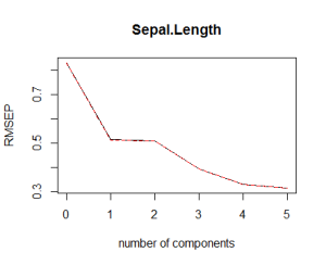
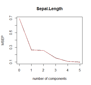
By default, the pcr function computes the root mean squared error and the validationplot function plots this statistic, however you can choose to plot the usual mean squared error or the R2
by setting the val.type argument equal to “MSEP” or “R2” respectively
|
1 2 |
# Plot the root mean squared error validationplot(pcr_model) |

|
1 2 |
# Plot the cross validation MSE validationplot(pcr_model, val.type="MSEP") |

|
1 2 |
# Plot the R2 validationplot(pcr_model, val.type = "R2") |

What you would like to see is a low cross validation error with a lower number of components than the number of variables in your dataset. If this is not the case or if the smalles cross validation error occurs with a number of components close to the number of variables in the original data, then no dimensionality reduction occurs. In the example above, it looks like 3 components are enough to explain more than 90% of the variability in the data although the CV score is a little higher than with 4 or 5 components. Finally, note that 6 components explain all the variability as expected.
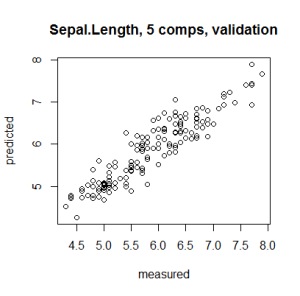
You can plot the predicted vs measured values using the predplot function as below
|
1 |
predplot(pcr_model) |

while the regression coefficients can be plotted using the coefplot function
|
1 |
coefplot(pcr_model) |

Now you can try to use PCR on a traning-test set and evaluate its performance using, for example, using only 3 components.
|
1 2 3 4 5 6 7 8 9 |
# Train-test split train <- iris[1:120,] y_test <- iris[120:150, 1] test <- iris[120:150, 2:5] pcr_model <- pcr(Sepal.Length~., data = train,scale =TRUE, validation = "CV") pcr_pred <- predict(pcr_model, test, ncomp = 3) mean((pcr_pred - y_test)^2) |
|
1 |
## [1] 0.213731 |
With the iris dataset there is probably no need to use PCR, in fact, it may even be worse using it. However, I hope this toy example was useful to introduce this model.
Thank you for reading this article, please feel free to leave a comment if you have any questions or suggestions and share the post with others if you find it useful.
More questions?
If you want to know more about PCR and other Data Mining techniques, check out the content of the Data Mining with R Course


[…] This article was originally posted on Quantide blog – see here. […]
[…] This article was originally posted on Quantide blog – see here. […]
[…] in R, an operational tutorial”, by John Mount, on the Revolutions blog; and this post, “Performing principal components regression (PCR) in R”, by Michy Alice, on the […]
[…] of the blue I decided to run PCA on the normalized dataset and found an interesting results worth […]
Hello,
For this ‘pls’ package, does the pcr function uses the “y-aware” method? or purely looking at x-only PCA generation?
Hi, I’m not sure about that since there is no mention of y-aware method in the official documentation.