Introduction
R is an object-oriented (OO) language. This basically means that R is able to recognize the type of objects generate from analysis and to apply the right operation on different objects.
For example, the summary(x) method performs different operations depending on the so-called “class” of x:
|
1 2 |
x <- data.frame(first=1:10, second=letters[1:10]) class(x) # An object of class "data.frame" |
|
1 |
## [1] "data.frame" |
|
1 |
summary(x) |
|
1 2 3 4 5 6 7 8 |
## first second ## Min. : 1.00 a :1 ## 1st Qu.: 3.25 b :1 ## Median : 5.50 c :1 ## Mean : 5.50 d :1 ## 3rd Qu.: 7.75 e :1 ## Max. :10.00 f :1 ## (Other):4 |
|
1 2 3 |
ds <- data.frame(x=1:100, y=100 + 3 * 1:100 + rnorm(100,sd = 10)) md <- lm(formula = y ~ x, data = ds) class(md) # An object of class "lm" |
|
1 |
## [1] "lm" |
|
1 |
summary(md) |
|
1 2 3 4 5 6 7 8 9 10 11 12 13 14 15 16 17 18 |
## ## Call: ## lm(formula = y ~ x, data = ds) ## ## Residuals: ## Min 1Q Median 3Q Max ## -20.1695 -5.8434 -0.4058 5.3611 27.9861 ## ## Coefficients: ## Estimate Std. Error t value Pr(>|t|) ## (Intercept) 100.07892 1.99555 50.15 <2e-16 *** ## x 2.98890 0.03431 87.12 <2e-16 *** ## --- ## Signif. codes: 0 '***' 0.001 '**' 0.01 '*' 0.05 '.' 0.1 ' ' 1 ## ## Residual standard error: 9.903 on 98 degrees of freedom ## Multiple R-squared: 0.9873, Adjusted R-squared: 0.9871 ## F-statistic: 7590 on 1 and 98 DF, p-value: < 2.2e-16 |
the outputs reported, and the calculations performed, by the summary() method are really different for the x and the mdobjects.
This behavior is one of characteristics of OO languages, and it is called methods overloading.
The methods overloading can be applied not only for methods in “function form” (i.e., for methods like summary()), but also for operators; indeed, “behind the scenes”, the operators are functions/methods. For example, if we try to write +
|
1 |
`+` |
|
1 |
## function (e1, e2) .Primitive("+") |
That means that the + operator actually is a function/method that requires two arguments: e1 and e2, which are respectively the left and right argument of operator itself.
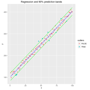
The + operator is present in R base, and can be overloaded as well, like in ggplot2 package, where the + operator is used to “build” the graph characteristics, as in following example:
|
1 2 3 4 5 6 7 8 9 10 11 12 13 |
require(ggplot2) prds <- predict(object = md, interval = "prediction", level=.9) ds <- cbind(ds, prds) ds$outliers <- as.factor(ds$y<ds$lwr | ds$y>ds$upr) graph <- ggplot(data = ds,mapping = aes(x=x, y=y, color=outliers)) graph <- graph + geom_point() graph <- graph + geom_line(aes(y=fit), col="blue") graph <- graph + geom_line(aes(y=lwr), col="green") graph <- graph + geom_line(aes(y=upr), col="green") graph <- graph + ggtitle("Regression and 90% prediction bands") print(graph) |

The + operator, then, is applied differently with ggplot2 objects (with respect other object types), where it “concatenates” or “assembles” parts of final graph.
In this small post, and following ones, I would like to produce some “jokes” with objects, operators, overloading, and similar “amenities”..
C-language += operator and its emulation in R
In C language there are several useful operators that allow the programmer to save some typing and to produce some more efficient and easiest to read code. The first operator that I would like to discuss is the += one.
+= is an operator that does operations like: a = a + k.
In C, the above sentence can be summarized with a += k. Of course, the sentence can be something of more complex, like
a += (x-log(2))^2
In this case, the code line shall be “translated” to a = a + (x-log(2))^2.
If I would like to have in R a new operator that acts similarly to C’s +=, I whould have to create it.
Unfortunately, not all the names are allowed in R for new operators: if I want to produce a new operator name I can only use operators with names like %mynewoperator% where the % symbols are mandatory.
Indeed, for this example, I will create a new %+=% operator that acts similarly to the C’s +=.
This new operator has to be able to get the values of variables passed as arguments, to sum them, and then, more importantly, to update the value of the first variable with the new value.
The first version of the new operator can be the following:
|
1 2 3 4 5 6 7 8 9 10 11 12 13 |
`%+=%` <- function(x,y){ # retreieve the first argument variable name var_name <- deparse(substitute(x)) # retrieve the environment where the %+=% has been used env <- parent.env(environment()) # calculate the sum sm <- x+y # save into the env environment the result of sum into the assign(x=var_name,value = sm,envir = env) } |
The function retrieves the name of variable to update by deparsing the x input variable (first argument of operator), and then calculates the sum between the first argument and the second argument values.
Finally, the function assigns the result of sum to the variable whose name has been previously retrieved, but in the environment from which the %+=% operator has been called (the environment is found at the line env <- parent.env(environment())).
Let’s test the operator:
|
1 2 3 |
a <- 10 a %+=% 15 a |
|
1 |
## [1] 25 |
It works!
Now a more complex test:
|
1 2 3 4 |
a <- 10 b <- log(2) a %+=% b a |
|
1 |
## [1] 10.69315 |
It works fine as well.
Now a more sophisticated test
|
1 2 3 4 5 6 7 |
graph <- ggplot(data = ds,mapping = aes(x=x, y=y, color=outliers)) graph %+=% geom_point() graph %+=% geom_line(aes(y=fit), col="blue") graph %+=% geom_line(aes(y=lwr), col="green") graph %+=% geom_line(aes(y=upr), col="green") graph %+=% ggtitle("Regression and 90% prediction bands") print(graph) |

It works correctly!
It seems that the new operator works as expected. It recognizes the object type and applies the correct method to different object types.
Some benchmarks
To test the performance of new operator, we need the microbenchmark library.
|
1 |
require(microbenchmark) |
|
1 |
## Loading required package: microbenchmark |
Now, we can test the new operator versus the “standard” operator. Let’s try with a simple summation:
|
1 2 3 |
aa <- 1 bb <- 1 microbenchmark(aa %+=% 1, bb <- bb+1,times = 10000) |
|
1 2 3 4 |
## Unit: nanoseconds ## expr min lq mean median uq max neval ## aa %+=% 1 13175 14813 16481.1057 15277 15792 1170934 10000 ## bb <- bb + 1 167 198 276.7191 255 300 20677 10000 |
Our new operator is about 60 times slower than the “base” operation!
Now we can test the same operator, but with more complex objects:
|
1 2 3 4 5 6 7 8 9 10 11 12 13 14 15 16 17 18 19 20 21 |
ggfunc_1 <- function(ds){ graph <- ggplot(data = ds,mapping = aes(x=x, y=y, color=outliers)) graph <- graph + geom_point() graph <- graph + geom_line(aes(y=fit), col="blue") graph <- graph + geom_line(aes(y=lwr), col="green") graph <- graph + geom_line(aes(y=upr), col="green") graph <- graph + ggtitle("Regression and 90% prediction bands") return(graph) } ggfunc_2 <- function(ds){ graph <- ggplot(data = ds,mapping = aes(x=x, y=y, color=outliers)) graph %+=% geom_point() graph %+=% geom_line(aes(y=fit), col="blue") graph %+=% geom_line(aes(y=lwr), col="green") graph %+=% geom_line(aes(y=upr), col="green") graph %+=% ggtitle("Regression and 90% prediction bands") return(graph) } |
The two above functions draw the same graph, but the first uses the “base” + operator, whereas the second one uses the%+=% operator. Let’s compare them:
|
1 |
microbenchmark(ggfunc_1(ds), ggfunc_2(ds),times = 1000) |
|
1 2 3 4 |
## Unit: milliseconds ## expr min lq mean median uq max neval ## ggfunc_1(ds) 4.665298 4.808219 5.214841 4.879535 5.038604 45.77439 1000 ## ggfunc_2(ds) 4.628490 4.763513 5.139376 4.836035 4.960999 45.46439 1000 |
In this case, the function with new operator performs like (if not better than) the function that uses the “standard” notations.
Conclusions
We played with environments, and operators, and we created a new operator that “simulates” the C’s += one.
This new operator allows the developer to reduce the code typing activity. Of course, by using a shorter name (for example, %+%) we can reduce again the typing.
As we created the += operator, we can build other operators like %-=%, %*=%, %/=%, and so on.
Now some considerations about performances: if we compare the new operator with the standard +-based coding applied on “base” objects, it results very slow; but if we compare the new operator with the + operator applied to more complex objects (in our example, a ggplot2 one), the new operator does not perform worse than the standard coding.
More enhancements can also be applied to code optimimzations, but I think that for this example the above code is good enough.
In future posts, I will deepen some aspects of overloading, C operators and classes.


[…] This post was originally posted on Quantide blog. Read the full article here. […]
[…] This post was originally posted on Quantide blog. Read the full article here. […]