
This article is the first chapter of Quantide’s web book “Raccoon – Statistical Models with R“. Raccoon is Quantide’s third web book after “Rabbit – Introduction to R” and “Ramarro – R for Developers“. See the full project here.
This chapter is an introduction to the first section of the book, Linear Models, and contain some theoretical explanation and lots of examples. At the end of the chapter you will find two summary tables with Linear model formulae and functions in R and Common R functions for inference.
Introduction to Linear Models
ds dataframe contains height (in cm) weight (in Kg), and gender of a different young person.Now, one might want to find a simple (or smooth) numerical relation (a regression) between
height and weight measures, where weight will depend on height.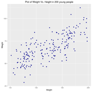
Relation between Weight and Height of 200 young people
In other words, one might want to draw a smooth line that “best approximates” the causal relation between height and weight (i.e., the height influences the weight).
Note that the relation might be really simple, as finding a simple “central value” (i.e., when one hypotesizes that weight does not change when varying the height); in this case the “best” smooth line could be the mean of weight values)
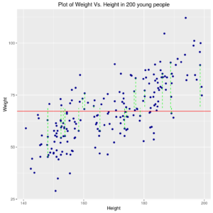
Relation between Weight and Height in 200 young people with ‘best constant model’ or the relation might be a few more complex, as a straight line of type (see next graph):
y=\(\beta_0\)+ \(\beta_1\)\( \cdot x \)
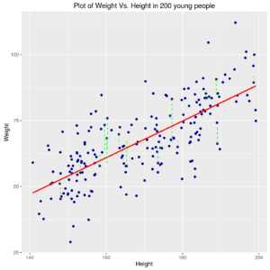
Relation between Weight and Height in 200 young people with best straight line model or also more complex.
Anyway, in either above cases the line is estimated by using the so-called “least squares” method: the “best” line is the one for which the sum of squares of differences between the points and line itself is minimum.
In first model, the “level” for which one can obtain the minimum of sum of squares of distance of points from line is at the average of weight values \((\overline{y}\)). The dashed green lines represent the distances of some observed points from the “best” (estimated) line.
In second model, the result of application of least-squares method is a few more complex, but can be obtained in closed form, as:
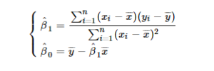
where \(\hat\beta_0\) and \(\hat\beta_1\) represent, respectively, the estimates of \(\beta_0\) and \(\beta_1\), \(n\) is the number of people in sample (the sample size), and \(\overline{x}\) and \(\overline{y}\) represent, respectively, the arithmetic mean of height and the arithmetic mean of weight values.
The least-squares method may be seen as a particular case of the more general Maximum Likelihood method to data for which the Normality assumption may be applied (see “Some theory on Linear Models” chapter).
However notice that least-squares method by itself does not give information about the “better” model: in above examples, least-squares estimates are available for the “only-mean” model as well as for the straight line model, but no information about the preferable model is returned by the least-squares. Some tests can be used to choose the best model (in next chapters we will give information about that).
Finally, the relation can be more complex again: for example, a different line for male and female people may be estimated (see next Figure).
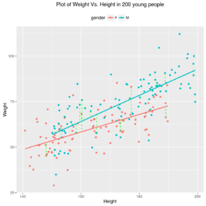
Relation between Weight and Height in 100 male and 100 female young people
This is because, roughly speaking, a model is said a linear model if unknown parameters and error term combine linearly, and not necessarily if the functional form, or relation, between independent and dependent variables is linear. In “Some Theory on Linear Model” chapter this topic is covered more thoroughly.
Linear model formulae and functions in R
There are lots of different types of regression models in statistics but R mantains a coherent syntax for the estimation of all of them. Indeed, the common interface to fit a model in R is made of a call to the corresponding function with arguments formula and data.
Talking about linear regression models, the lm and aov functions are used in R to fit respectively linear regression and analysis of variance model and their syntax is:
formula argument is a symbolic description of the model to be fitted, which has the form: response variable ∼ predictor variables. The variables involved in formula should be columns of a dataframe specied in data argument.
For example, consider ds dataset.
To fit a linear model on the relation between weight and height of ds dataset, the sintax is:
In the following table some formulas examples are shown, where y represents the response variable, x, x1, x2, x3 represent continuous variates, whereas upper case letters represent factors:
| Expression | Description |
|---|---|
y ~ x |
Simple regression |
y ~ 1 + x |
Explicit intercept |
y ~ -1 + x |
Through the origin |
y ~ x + I(x^2) |
Quadratic regression |
y ~ x1 + x2 + x3 |
Multiple regression |
y ~ G + x1 + x2 |
Parallel regressions |
y ~ G / (x1 + x2) |
Separate regressions |
sqrt(y) ~ x + I(x^2) |
Transformed |
y ~ G |
Single classification |
y ~ A + B |
Randomized block |
y ~ B + N * P |
Factorial in blocks |
y ~ x + B + N * P |
with covariate |
y ~ . -x1 |
All variables except x1 |
y ~ . + A:B |
Add interaction (update) |
Nitrogen ~ Times*(River/Site) |
More complex design |
The items in Expression column show several examples of formulas.
An expression of the form y ~ model is interpreted as a specification that the response y is modelled by a linear predictor specified symbolically by model. Such a model consists of a series of terms separated by + operators.
In next chapters, many examples of use of these functions will be then presented.
Common R functions for inference
In following table the main functions used for linear model analysis are presented.
All the functions have to be applied on objects of class lm or class aov, obtained by calling, respectively,
obj <- lm(formula) or obj <- aov(formula)
| Expression | Description |
|---|---|
coef(obj) |
regression coefficients |
resid(obj) |
residuals |
fitted(obj) |
fitted values |
summary(obj) |
analysis summary |
predict(obj, newdata = ndat) |
predict for newdata |
deviance(obj) |
residual sum of squares |

install.packages(“qdata”)
Warning in install.packages :
package ‘qdata’ is not available (for R version 3.3.1) — I would like to try your chapter 1 but I can’t!
Thank you Wayne for your comment. We forgot to publish the qdata package, but now it is available at Quantide’s Github page (https://github.com/quantide/qdata), as Arvins Betrabet noticed. It is a package containing about 80 dataset, that we will widely use throughout the web-book. We’ll add a direct link at the beginning of each chapter. Thanks!
The “qdata” package is on Quantide’s Github page
https://github.com/quantide/qdata
with Instructions on installing it with “devtools”
You found it! Thank you Arvind, it is absolutely right