Raccoon | Ch 2.4 - 3-way Anova - Quantide

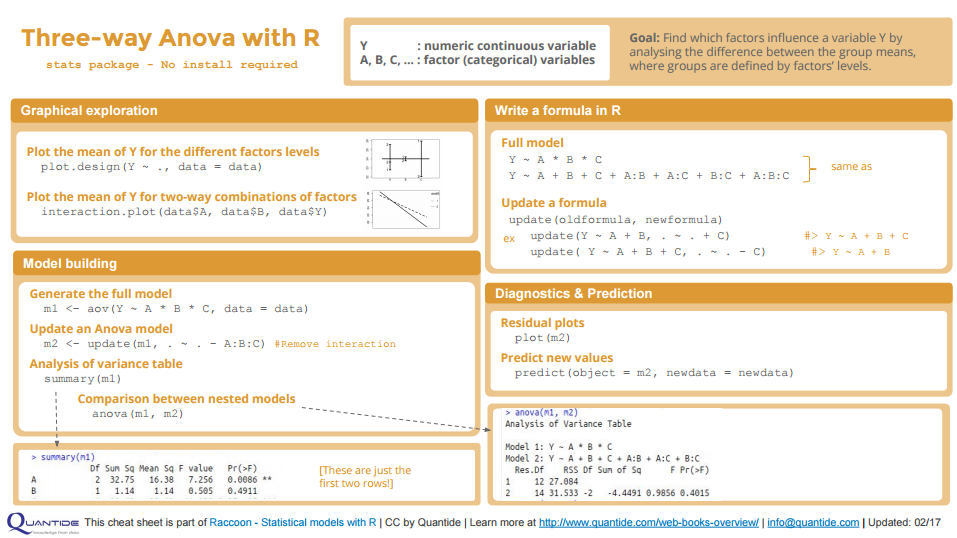
Download the 3-way Anova cheat sheet in full resolution: 3-way Anova with R cheat sheet

This article is part of Quantide’s web book “Raccoon – Statistical Models with R“. Raccoon is Quantide’s third web book after “Rabbit – Introduction to R” and “Ramarro – R for Developers“. See the full project here.

The second chapter of Raccoon is focused on T-test and Anova. Through example it shows theory and R code of:

1-sample t-test
2-sample t-test and Paired t
1-way Anova
3-way Anova
Unbalanced and Nested Anova

This post is the fourth section of the chapter, about 3-way Anova.

Throughout the web-book we will widely use the package qdata, containing about 80 datasets. You may find it here: https://github.com/quantide/qdata.

Example: Braking distances (3-way ANOVA)

Data description

Distance data contain measurements of braking distances on the same car equipped with several configurations of:

Tire: Factor with 3 levels GT, LS, MX
Tread: Factor with 2 levels 1.5, 10
ABS: Factor with levels disabled,enabled

For each combination of levels of the above three factors, 2 measurements of brake distance have been registered.

The objective of the experiment is to find which factor(s) influence the brake distance, and in which direction.

Data loading

data(distance)
head(distance)

1 2	data(distance) head(distance)

## # A tibble: 6 × 4
##     Tire  Tread      ABS Distance
##   <fctr> <fctr>   <fctr>    <dbl>
## 1     GT     10  enabled 19.35573
## 2     GT    1.5 disabled 23.38069
## 3     MX    1.5  enabled 24.00778
## 4     MX     10  enabled 25.07142
## 5     LS     10 disabled 26.39833
## 6     GT     10  enabled 18.60888

## # A tibble: 6 × 4

## Tire Tread ABS Distance

## <fctr> <fctr> <fctr> <dbl>

## 1 GT 10 enabled 19.35573

## 2 GT 1.5 disabled 23.38069

## 3 MX 1.5 enabled 24.00778

## 4 MX 10 enabled 25.07142

## 5 LS 10 disabled 26.39833

## 6 GT 10 enabled 18.60888

str(distance)

1	str(distance)

## Classes 'tbl_df', 'tbl' and 'data.frame':    24 obs. of  4 variables:
##  $ Tire    : Factor w/ 3 levels "GT","LS","MX": 1 1 3 3 2 1 2 2 2 3 ...
##  $ Tread   : Factor w/ 2 levels "1.5","10": 2 1 1 2 2 2 1 1 2 2 ...
##  $ ABS     : Factor w/ 2 levels "disabled","enabled": 2 1 2 2 1 2 2 1 1 1 ...
##  $ Distance: num  19.4 23.4 24 25.1 26.4 ...

## Classes 'tbl_df', 'tbl' and 'data.frame': 24 obs. of 4 variables:

## $ Tire : Factor w/ 3 levels "GT","LS","MX": 1 1 3 3 2 1 2 2 2 3 ...

## $ Tread : Factor w/ 2 levels "1.5","10": 2 1 1 2 2 2 1 1 2 2 ...

## $ ABS : Factor w/ 2 levels "disabled","enabled": 2 1 2 2 1 2 2 1 1 1 ...

## $ Distance: num 19.4 23.4 24 25.1 26.4 ...

Descriptives

Let us first get a graphical insight of the data. We want to graphically explore how the average braking distance changes given specific levels of the factors considered. Thus we first plot the univariate effects.

plot.design(Distance ~ ., data = distance)

1	plot.design(Distance ~ ., data = distance)

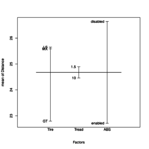
Plot of univariate factors effects on Distance response variable

The mean of the braking distance seems to change mainly with Tire type and ABS levels, while different levels of Tread seem to not influence the mean braking distance.

It may be interesting however to see whether different combinations of the levels of the factors differently affect the average braking distance. We could for example see whether a specific type of tire, combined with a specific level of tread affect the braking distance. Thus, let us plot the two-way interactions.

op <- par(mfrow = c(3, 1))
with(distance, {
  interaction.plot(ABS, Tire, Distance)
  interaction.plot(ABS, Tread, Distance)
  interaction.plot(Tread, Tire, Distance)
  }
)
par(op)

op <- par(mfrow = c(3, 1))

with(distance, {

interaction.plot(ABS, Tire, Distance)

interaction.plot(ABS, Tread, Distance)

interaction.plot(Tread, Tire, Distance)

}

)

par(op)

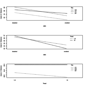
Plots of two-way interaction effects of factors on Distance response variable

The braking distance seems to decrease when ABS is enabled as compared to ABS disabled independently of the tire type (no interaction). However, there may be an interaction between Tread and ABS, that means that ABS might affect the braking distance differently based on whether it is combined with a specific type of tire.

So far we have commented on plots based on descriptive statistics only. In order to say whether the differences between the several means plotted are significant or not, we need to insert these factors in a model and run tests on each factor/interaction included in the model.

Inference and models of 3-way Anova

Let’s build a full model, that is the model with the three factors considered, the two-way interactions between all factors and the three-way interaction:

fm <- aov(Distance ~ ABS * Tire * Tread, data = distance)

1	fm <- aov(Distance ~ ABS * Tire * Tread, data = distance)

Notice that this is equivalent to writing:

fm <- aov(Distance ~ ABS + Tire + Tread + ABS:Tire + ABS:Tread + Tire:Tread
         + ABS:Tire:Tread, data = distance)
summary(fm)

fm <- aov(Distance ~ ABS + Tire + Tread + ABS:Tire + ABS:Tread + Tire:Tread

+ ABS:Tire:Tread, data = distance)

summary(fm)

##                Df Sum Sq Mean Sq F value   Pr(>F)    
## ABS             1  92.62   92.62  41.038 3.37e-05 ***
## Tire            2  42.64   21.32   9.446  0.00344 ** 
## Tread           1   1.14    1.14   0.505  0.49108    
## ABS:Tire        2   9.60    4.80   2.127  0.16187    
## ABS:Tread       1   5.13    5.13   2.273  0.15748    
## Tire:Tread      2   2.08    1.04   0.462  0.64107    
## ABS:Tire:Tread  2   4.45    2.22   0.986  0.40149    
## Residuals      12  27.08    2.26                     
## ---
## Signif. codes:  0 '***' 0.001 '**' 0.01 '*' 0.05 '.' 0.1 ' ' 1

## Df Sum Sq Mean Sq F value Pr(>F)

## ABS 1 92.62 92.62 41.038 3.37e-05 ***

## Tire 2 42.64 21.32 9.446 0.00344 **

## Tread 1 1.14 1.14 0.505 0.49108

## ABS:Tire 2 9.60 4.80 2.127 0.16187

## ABS:Tread 1 5.13 5.13 2.273 0.15748

## Tire:Tread 2 2.08 1.04 0.462 0.64107

## ABS:Tire:Tread 2 4.45 2.22 0.986 0.40149

## Residuals 12 27.08 2.26

## ---

## Signif. codes: 0 '***' 0.001 '**' 0.01 '*' 0.05 '.' 0.1 ' ' 1

Only main effects ABS and Tire seem to influence the mean of the braking distance (similarly to what we had guessed by looking at the plots!). Interactions seem not significant, meaning that those differences we had noticed in the two-way interactions plots were too small to be statistically significant. We can now start to drop the interactions from the three-way interaction.

In general we are interested in finding the most provident model which better explains the variability in the data. Once the full model has been fitted, we start by dropping the highest-level interactions because we “move” within the hierarchical models paradigm.

To obtain the model without three-way interaction, we can use update():

fm <- update(fm, . ~ . -ABS:Tire:Tread)
summary(fm)

1 2	fm <- update(fm, . ~ . -ABS:Tire:Tread) summary(fm)

##             Df Sum Sq Mean Sq F value   Pr(>F)    
## ABS          1  92.62   92.62  41.123 1.62e-05 ***
## Tire         2  42.64   21.32   9.465  0.00251 ** 
## Tread        1   1.14    1.14   0.506  0.48873    
## ABS:Tire     2   9.60    4.80   2.132  0.15552    
## ABS:Tread    1   5.13    5.13   2.278  0.15345    
## Tire:Tread   2   2.08    1.04   0.462  0.63902    
## Residuals   14  31.53    2.25                     
## ---
## Signif. codes:  0 '***' 0.001 '**' 0.01 '*' 0.05 '.' 0.1 ' ' 1

## Df Sum Sq Mean Sq F value Pr(>F)

## ABS 1 92.62 92.62 41.123 1.62e-05 ***

## Tire 2 42.64 21.32 9.465 0.00251 **

## Tread 1 1.14 1.14 0.506 0.48873

## ABS:Tire 2 9.60 4.80 2.132 0.15552

## ABS:Tread 1 5.13 5.13 2.278 0.15345

## Tire:Tread 2 2.08 1.04 0.462 0.63902

## Residuals 14 31.53 2.25

## ---

## Signif. codes: 0 '***' 0.001 '**' 0.01 '*' 0.05 '.' 0.1 ' ' 1

Since two ways interactions seem to not affect the mean braking distance, we could now try to remove all two-way interactions, always using update() function:

fm1 <- update(fm, .~ABS+Tire+Tread)
summary(fm1)

1 2	fm1 <- update(fm, .~ABS+Tire+Tread) summary(fm1)

##             Df Sum Sq Mean Sq F value   Pr(>F)    
## ABS          1  92.62   92.62  36.397 8.37e-06 ***
## Tire         2  42.64   21.32   8.377  0.00246 ** 
## Tread        1   1.14    1.14   0.447  0.51157    
## Residuals   19  48.35    2.54                     
## ---
## Signif. codes:  0 '***' 0.001 '**' 0.01 '*' 0.05 '.' 0.1 ' ' 1

## Df Sum Sq Mean Sq F value Pr(>F)

## ABS 1 92.62 92.62 36.397 8.37e-06 ***

## Tire 2 42.64 21.32 8.377 0.00246 **

## Tread 1 1.14 1.14 0.447 0.51157

## Residuals 19 48.35 2.54

## ---

## Signif. codes: 0 '***' 0.001 '**' 0.01 '*' 0.05 '.' 0.1 ' ' 1

The result is not surprising, as it is very similar to that found with the previous models. It is better to check if the three removed effects together are still not significant using anova():

anova(fm, fm1)

1	anova(fm, fm1)

## Analysis of Variance Table
## 
## Model 1: Distance ~ ABS + Tire + Tread + ABS:Tire + ABS:Tread + Tire:Tread
## Model 2: Distance ~ ABS + Tire + Tread
##   Res.Df    RSS Df Sum of Sq      F Pr(>F)
## 1     14 31.533                           
## 2     19 48.351 -5   -16.818 1.4933 0.2539

## Analysis of Variance Table

## Model 1: Distance ~ ABS + Tire + Tread + ABS:Tire + ABS:Tread + Tire:Tread

## Model 2: Distance ~ ABS + Tire + Tread

## Res.Df RSS Df Sum of Sq F Pr(>F)

## 1 14 31.533

## 2 19 48.351 -5 -16.818 1.4933 0.2539

The combined effect of the three-way interactions is not significant, thus we can continue on with the model with the main effects only.
The tables of effects from model follow below

model.tables(fm1,type="effects")

1	model.tables(fm1,type="effects")

## Tables of effects
## 
##  ABS 
## ABS
## disabled  enabled 
##   1.9645  -1.9645 
## 
##  Tire 
## Tire
##      GT      LS      MX 
## -1.8846  0.9755  0.9091 
## 
##  Tread 
## Tread
##      1.5       10 
##  0.21783 -0.21783

## Tables of effects

## ABS

## disabled enabled

## 1.9645 -1.9645

## Tire

## GT LS MX

## -1.8846 0.9755 0.9091

## Tread

## 1.5 10

## 0.21783 -0.21783

And now the table of means from model

model.tables(fm1,type="means")

1	model.tables(fm1,type="means")

## Tables of means
## Grand mean
##          
## 24.67633 
## 
##  ABS 
## ABS
## disabled  enabled 
##   26.641   22.712 
## 
##  Tire 
## Tire
##     GT     LS     MX 
## 22.792 25.652 25.585 
## 
##  Tread 
## Tread
##    1.5     10 
## 24.894 24.459

## Tables of means

## Grand mean

## 24.67633

## ABS

## disabled enabled

## 26.641 22.712

## Tire

## GT LS MX

## 22.792 25.652 25.585

## Tread

## 1.5 10

## 24.894 24.459

Finally, we remove the Tread effect to obtain the final model with significant effects only:

fm <- aov(Distance ~ ABS + Tire, data = distance)
summary(fm)

1 2	fm <- aov(Distance ~ ABS + Tire, data = distance) summary(fm)

##             Df Sum Sq Mean Sq F value   Pr(>F)    
## ABS          1  92.62   92.62  37.431 5.59e-06 ***
## Tire         2  42.64   21.32   8.615    0.002 ** 
## Residuals   20  49.49    2.47                     
## ---
## Signif. codes:  0 '***' 0.001 '**' 0.01 '*' 0.05 '.' 0.1 ' ' 1

## Df Sum Sq Mean Sq F value Pr(>F)

## ABS 1 92.62 92.62 37.431 5.59e-06 ***

## Tire 2 42.64 21.32 8.615 0.002 **

## Residuals 20 49.49 2.47

## ---

## Signif. codes: 0 '***' 0.001 '**' 0.01 '*' 0.05 '.' 0.1 ' ' 1

Residual analysis of 3-way Anova

op <-  par(mfrow = c(2, 2))
plot(fm)
par(op)

op <- par(mfrow = c(2, 2))

plot(fm)

par(op)

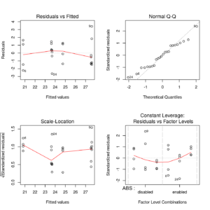
Compound residual plot for final brake distance model

Since the leverages are constant (as is typically the case in a balanced aov situation) the 4th plot draws factor level combinations instead of the leverages for the x-axis. (Notice that the factor levels are ordered by mean fitted value)

Distance means for each ABS and Tire category follow:

distance %>% group_by(ABS, Tire) %>% summarise(mean(Distance))

1	distance %>% group_by(ABS, Tire) %>% summarise(mean(Distance))

## Source: local data frame [6 x 3]
## Groups: ABS [?]
## 
##        ABS   Tire `mean(Distance)`
##     <fctr> <fctr>            <dbl>
## 1 disabled     GT         24.98647
## 2 disabled     LS         28.24991
## 3 disabled     MX         26.68618
## 4  enabled     GT         20.59702
## 5  enabled     LS         23.05378
## 6  enabled     MX         24.48464

## Source: local data frame [6 x 3]

## Groups: ABS [?]

## ABS Tire `mean(Distance)`

## <fctr> <fctr> <dbl>

## 1 disabled GT 24.98647

## 2 disabled LS 28.24991

## 3 disabled MX 26.68618

## 4 enabled GT 20.59702

## 5 enabled LS 23.05378

## 6 enabled MX 24.48464

While the table of grand means from model can be found as follows:

model.tables(fm, type="means")

1	model.tables(fm, type="means")

## Tables of means
## Grand mean
##          
## 24.67633 
## 
##  ABS 
## ABS
## disabled  enabled 
##   26.641   22.712 
## 
##  Tire 
## Tire
##     GT     LS     MX 
## 22.792 25.652 25.585

## Tables of means

## Grand mean

## 24.67633

## ABS

## disabled enabled

## 26.641 22.712

## Tire

## GT LS MX

## 22.792 25.652 25.585

Last we can get some predicted values from ANOVA model:

df_pred <- data.frame(ABS=c("enabled","disabled"),Tire=c("GT","LS"))
predict(object=fm,newdata=df_pred)

1 2	df_pred <- data.frame(ABS=c("enabled","disabled"),Tire=c("GT","LS")) predict(object=fm,newdata=df_pred)

##        1        2 
## 20.82722 27.61636

1 2	## 1 2 ## 20.82722 27.61636

Question: predicted values are different from the above calculated sampling averages. Why?

Raccoon | Ch 2.4 – 3-way Anova

Example: Braking distances (3-way ANOVA)

Data description

Data loading

Descriptives

Inference and models of 3-way Anova

Residual analysis of 3-way Anova

Join us!

Courses calendar

We are part of

Categories

Archives

Raccoon | Ch 2.4 – 3-way Anova

Example: Braking distances (3-way ANOVA)

Data description

Data loading

Descriptives

Inference and models of 3-way Anova

Residual analysis of 3-way Anova

Profile cancel

Join us!

Courses calendar

We are part of

Categories

Archives

Tags