Raccoon | Ch 2.5 – Unbalanced and Nested Anova

 

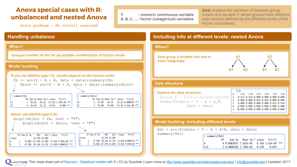
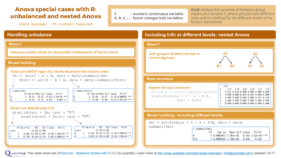
Download the Unbalanced and Nested Anova cheat sheet in full resolution: Anova special cases

This article is part of Quantide’s web book “Raccoon – Statistical Models with R“. Raccoon is Quantide’s third web book after “Rabbit – Introduction to R” and “Ramarro – R for Developers“. See the full project here.

The second chapter of Raccoon is focused on T-test and Anova. Through example it shows theory and R code of:

• 1-sample t-test
• 2-sample t-test and Paired t
• 1-way Anova
• 3-way Anova
• Unbalanced and Nested Anova

This post is the fifth section of the chapter, about Unbalanced Anova with one obs dropped and fixed effects Nested Anova.

Throughout the web-book we will widely use the package qdata, containing about 80 datasets. You may find it here: https://github.com/quantide/qdata.

Example: Brake distance 1 (unbalanced anova with one obs dropped)

Let us drop one observation so that all the factor levels combinations do not contain the same number of observations. We drop the observation with the values “LS 10 enabled”

Descriptives

As usual, we first plot the univariate effects:

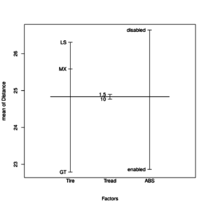Univariate effects plot of unbalanced model

Secondly we look at the two-way interaction plot:

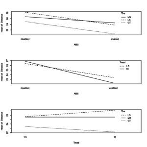
Two-way interaction effects plots of unbalanced model

We notice that all effects do not seem to change with respect to the previous example of 3-way anova.

Inference and models

In this section is where we’ll start noticing some differences with the balanced model. First let us fit the model with all interactions

As none of the interactions are significant, we drop them one by one, starting from the three-way interaction:

We continue on by dropping the two way interactions:

And we then make sure that the model without the interaction is actually better than that with interactions:

As expected, the model with interactions is not significantly better than that without interactions. 

The final model is hence the same as the model in the previous example of balanced Anova. However, notice that the sums of squares of the following two models (that we expect to be equal), are different:

Since aov() performs Type I SS ANOVA (we will see a wide explanation of Types of Sum of Squares in the Appendix) and this example uses data from unbalanced design, the previous 2 models give different results in terms of SS and respective p-values. In fact Type I SS ANOVA depends on the order in which factors are included in the model: fm is based on SS(ABS) and SS(Tire|ABS), whereas fminv is based on SS(Tire) and SS(ABS|Tire).

In order to avoid this problem, we may use Type II ANOVA: drop1() function allows to do this.

In this case, the results are equal. Alternatively, the function Anova() of the package car is available. Anova() allows Type II and III Sum of Squares too.

Notice that, until now, at least six types of sum of squares have been introduced in literature.
However, there are open discussions among statisticians about the use and pros/cons of different Types of SS.

Residual analysis

Together with the model results, one should always provide some statistics/plots on the residuals.

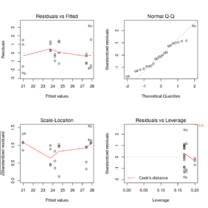
Residual plots of unbalanced model

In this case, since the leverages are not constant (unbalanced design) 4th plot draws the leverages in x-axis.

 

 

Example: Pin diameters (Fixed effects Nested ANOVA)

Data description

The dataframe considered in this example contains data collected from five different lathes, each of them used by two different operators. The goal of the study is to evaluate if significant differences in the mean diameter of pins occur between lathes and/or operators. Notice that here we are concerned with the effect of operators, so the layout of experiment is nested. If we were concerned with shift instead of operator, the layout would have been the other way around.

Data loading

Descriptives

Let us first carry out some descriptive statistics and plots in order to get a glimpse of the data. The next  few lines of code show descriptive statistics for each variable and the mean for each combination of Lathe and Operator factor levels.

Above statistics are not completely well-advised, since the operators working in the same part of the day (day or night) are different (nested anova) for different lathes. Let us draw a box-plot for each Late x Operator combination.

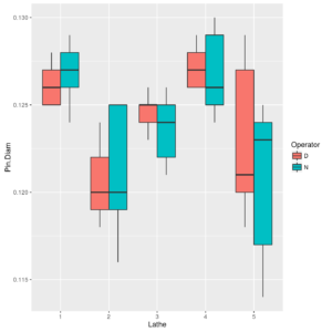
Boxplot of Pin.Diam by Lathe x Operator

It may seem natural to perform the following (incorrect) ANOVA to analyze diameters conditional on Lathe and Shift (i.e., considering Operator levels as equivalent to different shifts of working days) as for classical factorial layout.

The above results give however an incorrect model for the data under study. In fact the actual data structure is the following:

The correct ANOVA to perform is thus the following:

The / formula operator means that the levels of Operator factor are nested within the levels of Lathe factor. If we read the output we find that lathes seem to produce on average different products, whereas the difference between the means of the pins’ diameter conditional on the operator does not seem to be significant. Although the final results of the two Anovas (the first of which is incorrect and the second one correct!) may seem similar nested Anova is the one to use because there is a control over the variability given by the (fixed) effect of the operators. Nested Anova is hence useful for reducing the general variability of the plan and getting more significant differences among the levels of the factors.

An equivalent model formulation for nested ANOVA is given by:

or

Residuals analysis

Finally, residuals may be plotted for model’s diagnostics:

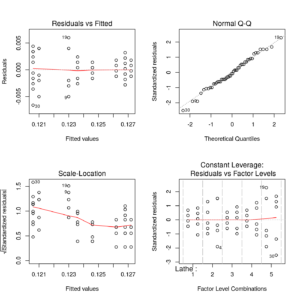
Residual plot of Late by Operator nested model